Introduction
In social sciences, variables of interest are often conceptualized as latent variables — hidden continuous variables measured through Likert scale questions, typically categorized as Strongly disagree, Disagree, Neutral, Agree, and Strongly agree. Researchers frequently aim to uncover these latent variables using various statistical techniques. Accurate modeling of survey data is essential for comparative analysis through simulation. The latent2likert package addresses this need by providing an effective algorithm to simulate Likert response variables from hypothetical latent variables. This vignette provides two practical workflow examples demonstrating the use of the latent2likert package.
Simulating Survey Data
The following hypothetical survey simulation is loosely based on an actual comparative study on teaching and learning R in a pair of introductory statistics labs (McNamara 2024).
Imagine a situation where 10 participants from Course A and 20 participants from Course B have completed the survey. Suppose the initial question was:
“How would you rate your experience with the course?”
with four possible answers:
Poor, Fair, Good, and Excellent.
Let’s assume that the participants in Course A were neutral regarding the question, while participants in Course B had a more positive experience on average.
By choosing appropriate parameters for the latent distributions and setting the number of categories n_levels = 4, we can generate hypothetical responses (standard deviation sd = 1 and skewness skew = 0, by default):
library(latent2likert) # Load the package
set.seed(12345) # Ensure reproducible results

# Generate responses for Course A and Course B
responses_A <- rlikert(size = 10, n_items = 1, n_levels = 4, mean = 0, sd = 1)
responses_B <- rlikert(size = 20, n_items = 1, n_levels = 4, mean = 1, sd = 1)
To summarize the results, create a data frame from all responses:
n_levels <- 4
n_groups <- 2
categories <- c("Poor", "Fair", "Good", "Excellent")

# Create a data frame to summarize the responses
response_data <- data.frame(
  Course = rep(c("A", "B"), each = n_levels),
  Response = factor(rep(categories, n_groups), levels = categories),
  Proportion = c(
    response_prop(responses_A, n_levels),
    response_prop(responses_B, n_levels)
  )
)

# Filter out rows with zero proportions
response_data <- response_data[response_data$Proportion > 0, ]
response_data
#>   Course  Response Proportion
#> 1      A      Poor       0.30
#> 2      A      Fair       0.20
#> 3      A      Good       0.20
#> 4      A Excellent       0.30
#> 6      B      Fair       0.10
#> 7      B      Good       0.25
#> 8      B Excellent       0.65
The results can then be visualized using a grouped bar chart:

Pre and Post Comparison
Now suppose that the survey also asked the participants to rate their skills on a 5-point Likert scale, ranging from 1 (very poor) to 5 (very good) in:
- Programming,
- Searching Online,
- Solving Problems.
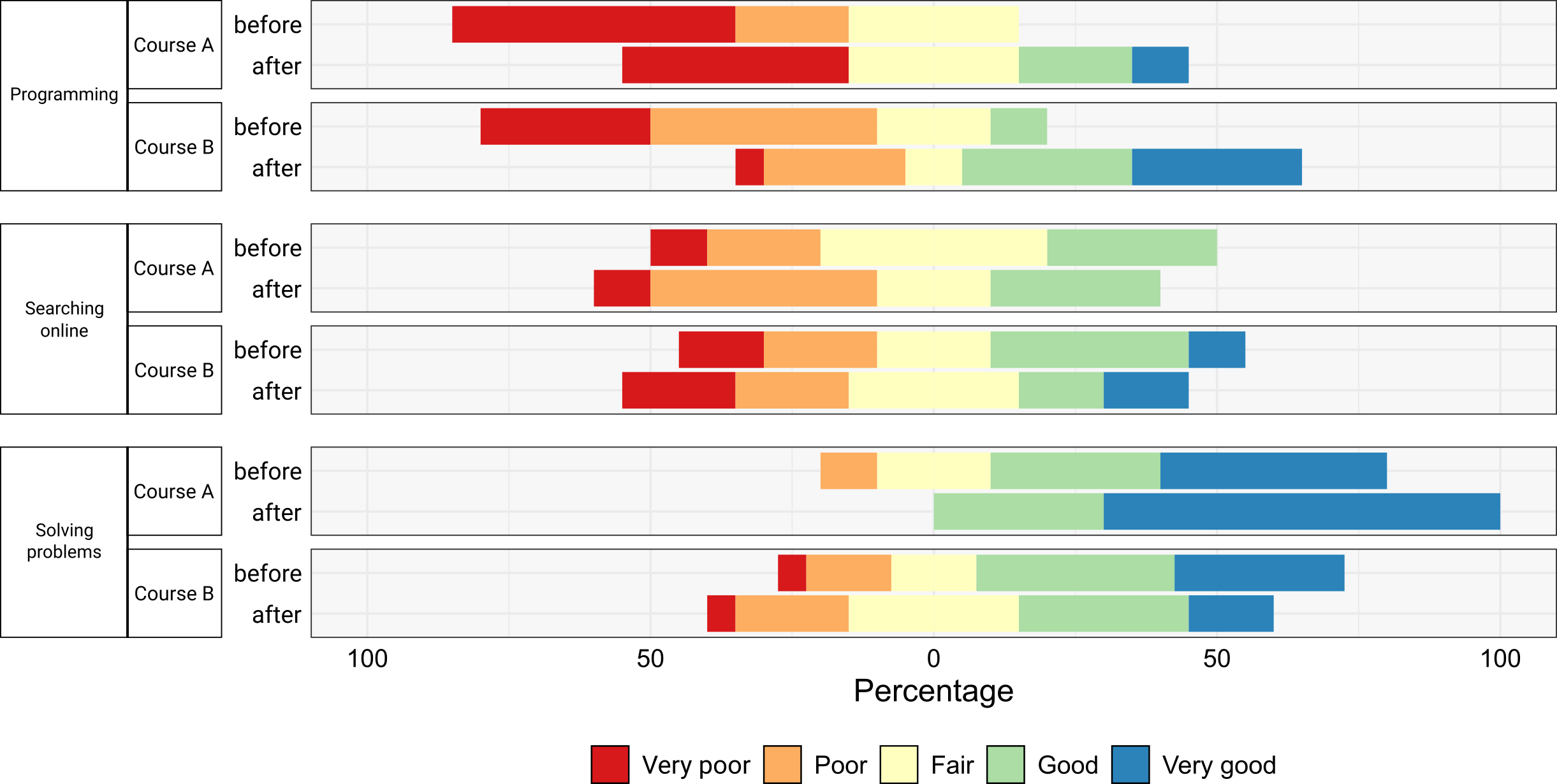
The survey was completed by the participants both before and after taking the course for a pre and post-comparison. Suppose that participants’ assessments of:
- Programming skills on average increased,
- Searching Online stayed about the same,
- Solving Problems increased in Course A, but decreased for participants in Course B.
Let’s simulate the survey data for this scenario:
# Pre- and post-assessments of skills for Course A
pre_A <- rlikert(size = 10, n_items = 3, n_levels = 5, mean = c(-1, 0, 1))
post_A <- rlikert(size = 10, n_items = 3, n_levels = 5, mean = c(0, 0, 2))

# Pre- and post-assessments of skills for Course B
pre_B <- rlikert(size = 20, n_items = 3, n_levels = 5, mean = c(-1, 0, 1))
post_B <- rlikert(size = 20, n_items = 3, n_levels = 5, mean = c(0, 0, 0))
Create a data frame from all responses to summarize the results:
# Combine pre and post responses into a list
pre_post <- list(pre_A, post_A, pre_B, post_B)

# Number of items and response levels
n_items <- 3
n_levels <- 5

# Define skills assessed
skills <- c("Programming", "Searching online", "Solving problems")

# Generate repeated skill labels for questions
questions <- rep(rep(skills, each = n_levels), 4)
questions <- factor(questions, levels = skills)

# Create a data frame to summarize the responses
response_data <- data.frame(
  Course = rep(c("Course A", "Course B"), each = 2 * n_items * n_levels),
  Question = questions,
  Time = as.factor(rep(c(
    rep("before", n_items * n_levels),
    rep("after", n_items * n_levels)
  ), 2)),
  Response = rep(seq_len(n_levels), 2 * n_items * 2),
  Proportion = as.vector(sapply(pre_post, function(d) {
    as.vector(t(response_prop(d, n_levels)))
  }))
)

head(response_data)
#>     Course         Question   Time Response Proportion
#> 1 Course A      Programming before        1        0.5
#> 2 Course A      Programming before        2        0.2
#> 3 Course A      Programming before        3        0.3
#> 4 Course A      Programming before        4        0.0
#> 5 Course A      Programming before        5        0.0
#> 6 Course A Searching online before        1        0.1
And visualize the results with a stacked bar chart:

Recreating Scale Scores
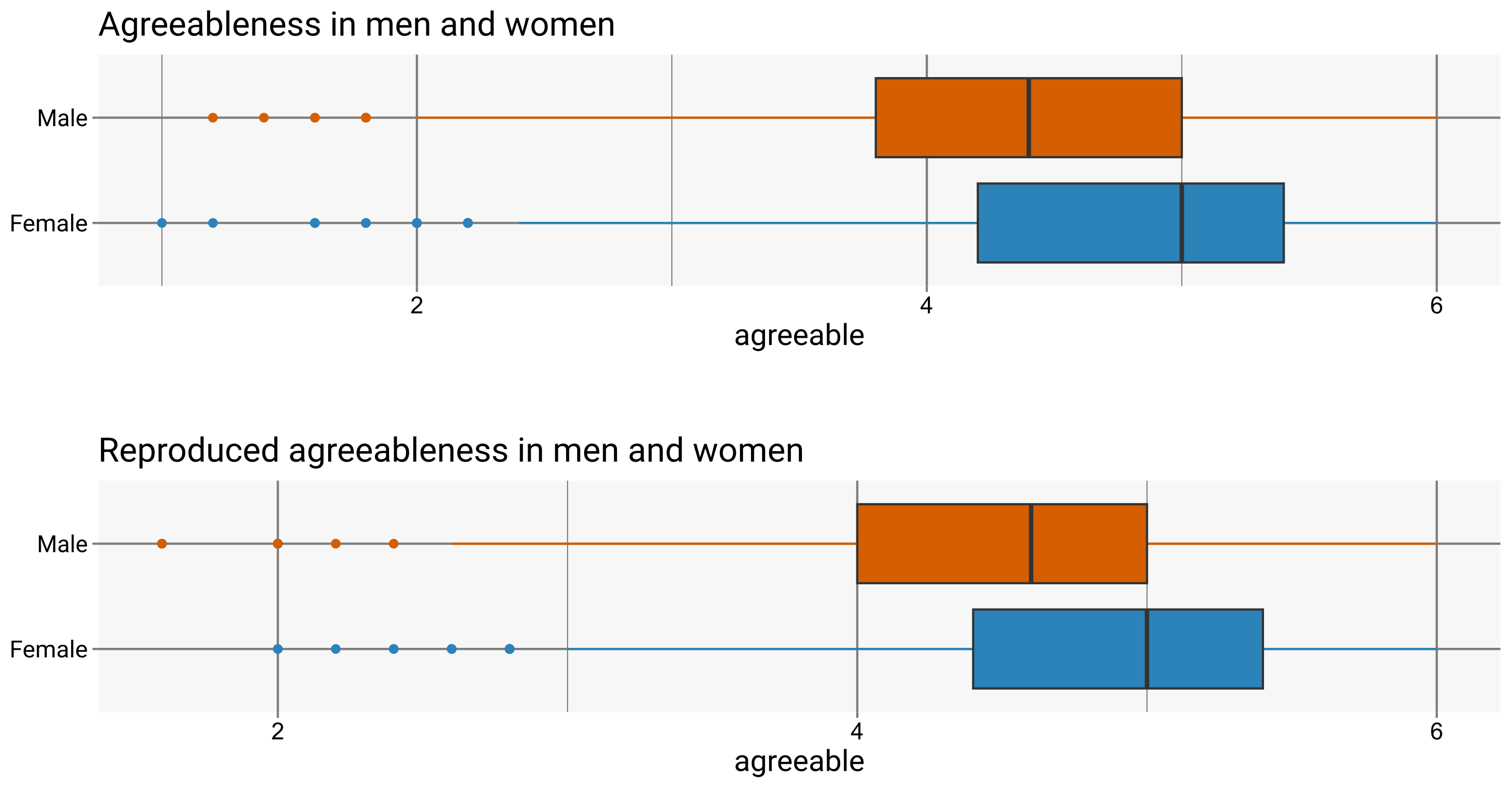
We will use part of the bfi data set from (Revelle 2024). Specifically, we’ll focus on the first 5 items corresponding to agreeableness. To investigate the differences in agreeableness between men and women, we’ll also use the gender attribute.
Load the data:
data(part_bfi)
head(part_bfi)
#>       A1 A2 A3 A4 A5 gender
#> 61617  2  4  3  4  4      0
#> 61618  2  4  5  2  5      1
#> 61620  5  4  5  4  4      1
#> 61621  4  4  6  5  5      1
#> 61622  2  3  3  4  5      0
#> 61623  6  6  5  6  5      1
Separate the items into two groups according to their gender:
vars <- c("A1", "A2", "A3", "A4", "A5")
items_male <- part_bfi[part_bfi$gender == 0, vars]
items_female <- part_bfi[part_bfi$gender == 1, vars]
Estimate the parameters of the latent variables, assuming they are
normal and providing the number of possible response categories
n_levels = 6:
params_male <- estimate_params(data = items_male, n_levels = 6)
params_female <- estimate_params(data = items_female, n_levels = 6)
Generate new responses to the items using the estimated parameters and estimated correlations:
set.seed(12345) # Ensure reproducible results

new_items_male <- rlikert(
  size = nrow(items_male),
  n_items = 5,
  n_levels = 6,
  mean = params_male["mean", ],
  sd = params_male["sd", ],
  corr = cor(items_male)
)

new_items_female <- rlikert(
  size = nrow(items_female),
  n_items = 5,
  n_levels = 6,
  mean = params_female["mean", ],
  sd = params_female["sd", ],
  corr = cor(items_female)
)
Create agreeableness scale scores for both groups of participants by taking the average of these 5 items:
# Combine new items and gender in new data frame
new_data <- data.frame(rbind(new_items_male, new_items_female))
new_data$gender <- c(rep(0, nrow(items_male)), rep(1, nrow(items_female)))
head(new_data)
#>   Y1 Y2 Y3 Y4 Y5 gender
#> 1  3  5  5  4  5      0
#> 2  1  5  4  4  4      0
#> 3  2  6  5  6  4      0
#> 4  4  4  4  6  5      0
#> 5  4  5  3  2  2      0
#> 6  5  4  5  6  5      0
# Reverse the first item because it has negative correlations
part_bfi$A1 <- (min(part_bfi$A1) + max(part_bfi$A1)) - part_bfi$A1
new_data$Y1 <- (min(new_data$Y1) + max(new_data$Y1)) - new_data$Y1

# Create agreeableness scale scores
part_bfi$agreeable <- rowMeans(part_bfi[, vars])
new_data$agreeable <- rowMeans(new_data[, c("Y1", "Y2", "Y3", "Y4", "Y5")])
The results can be visualized with a grouped boxplot:

